2018/12/24
【13.実践6】TinyYoloで物体検出

どうも、ディープなクラゲです。
「ゼロから学ぶディープラーニング推論」シリーズの13回目記事です。
このシリーズでは、Neural Compute StickとRaspberryPiの使い方をゼロから徹底的に学び、成果としてディープラーニングの推論アプリケーションが作れるようになることを目指しています。
第13回目は、TinyYoloで物体検出を行います。
具体的な実行方法とコードについて解説してゆきます
【 目次 】
- TinyYolo推論実行
- Yoloアルゴリズム
- TinyYolo推論コード解説
- (1) import関連
- (2) グローバル変数定義
- (3) main関数
- (4) filter_objects関数
- (5) boxes_to_pixel_units関数
- (6) get_duplicate_box_mask関数
- (7) get_intersection_over_union関数
- (8) display_objects_in_gui関数
TinyYolo推論実行
TinyYoloは「物体検出」が可能なモデルです
これまで実施してきたGoogLeNetやGenderNetなどの「画像認識」は1画像に対して1つの認識しか出来ませんでしたが、「物体検出」は1画像に対して複数の認識が可能となります。さらに、認識した物体の位置や大きさも知ることができます。
TinyYoloもSDKのサンプルソースには入ってはおらず、Neural Compute Application Zoo (NC App Zoo)にて公開されています。
NC App zooは第11回目のGenderNet/AgeNetで性別/年齢推定でgit cloneダウンロード済だと思います。
今回はTinyYoloをmakeしましょう
TinyYoloフォルダに移動して make します。数分で終わると思います。
cd ~/workspace/ncappzoo/caffe/TinyYolomake
run.pyを実行します
python3 run.py
ウィンドウが開いて次のような画像が出れば成功です
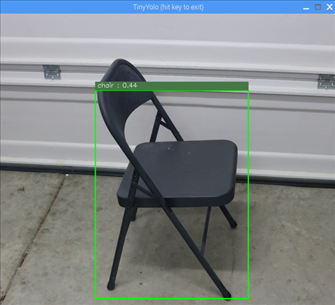
推論した画像は /home/pi/workspace/ncappzoo/data/images にある nps_chair.png です。
input_image_file= '../../data/images/nps_chair.png'
run.pyの13行目を変更すれば任意の画像で簡単に試せます
認識できる物体は以下の20種類です。
- aeroplane
- bicycle
- bird
- boat
- bottle
- bus
- car
- cat
- chair
- cow
- diningtable
- dog
- horse
- motorbike
- person
- pottedplant
- sheep
- sofa
- train
- tvmonitor
Yoloアルゴリズム
ここでは物体検出Yoloのアルゴリズムについてざっくりイメージで解説します。
Yolo以前の物体検出は、物体領域を検出してから各領域に対して画像認識を行うというアルゴリズムが主流でした。
それに対し、YOLO(You Only Look Once)は物体領域検出と画像認識を同時に行うというアルゴリズムで、従来の物体検出より速く行うことが可能です。ちなみに今回使用しているTiny版は、その名の通り小さなメモリで実行可能なモデルで、認識率よりも検出のスピードを重視しているようです。
物体領域検出は以下のような感じで表現されます。
それぞれの矩形はバウンディングボックス(BB)と呼ばれていて、その領域検出の信用度が高いほど太い枠で表示されています。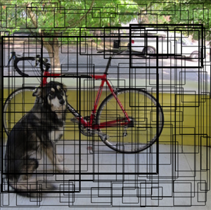
https://pjreddie.com/
Yolo以前のアルゴリズムでは、各BBについてCNNによる画像認識を行うという手法でした。
CNNによる画像認識は処理時間がかかりますので、できるだけ回数を減らした方が良いです。
そこでYoloは、BBに関係なく画像を7×7のセルに分割し、各セル49箇所に対してのみCNN画像認識を行っています。
また、BBは各セルに対して候補を2個だけに絞っています。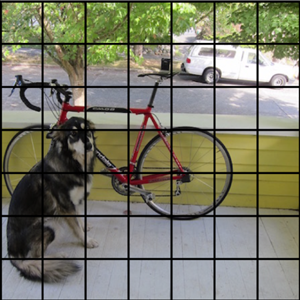
https://pjreddie.com/
各セルに対してのみCNN画像認識を行うイメージは以下の通りです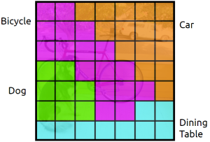
https://pjreddie.com/
各セルの2個のBBに対し、先ほどの画像認識の結果を融合すると以下のようなイメージで成果物が得られます
ここまでディープラーニングを使って一気通貫で処理されます。
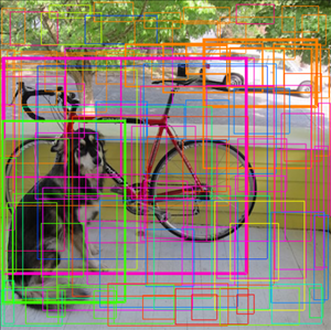
このままだと非常に情報量の多い表示となってしまいます。そこで、その後プログラミングですっきりさせる処理を行います。
閾値設定に基づき、信用度の高いところのみを抜き出し、重複箇所を消します。
すると、こんな感じで「すっきりした情報」になります。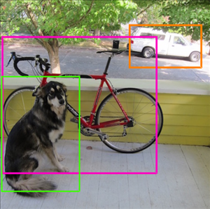
https://pjreddie.com/
今回の推論コードでは、このすっきりさせる部分がほとんどを占めています。では推論コードをじっくり見てゆきましょう!
TinyYolo推論コード解説
ソースコード全体はこちらからも見られます
https://github.com/movidius/ncappzoo/blob/ncsdk2/caffe/TinyYolo/run.py
まず、全体のざっくり構成を見てゆきましょう
(1) import関連(2) グローバル変数定義(4) filter_objects関数(6) get_duplicate_box_mask関数(5) boxes_to_pixel_units関数(7) get_intersection_over_union関数(8) display_objects_in_gui関数(3) main関数
関数など大きなまとまりで分けるとこのような構成になっています。
先頭の番号の意味は実行順番です。
(1)(2)以外は全て関数です。
プログラムの一番最後に以下の記述がありますが、これはPython基礎で学んだ内容です。忘れた人は見返してみましょう。
if __name__ == "__main__":sys
簡単に言うとmain関数から始めるという意味になります。
つまり、main関数が全ての関数の中で一番最初に実行されるということになります。
それでは実行順に、それぞれの詳細内容をじっくり見てゆきます!
今回はかなりボリュームがあります。忙しい人は、とりあえずmain関数の解説だけを見れば全体が分かると思います。
(1) import関連
#! /usr/bin/env python3# Copyright(c) 2017 Intel Corporation.# License: MIT See LICENSE file in root directory.
ここは問題ないですね。1行目はお決まりコードで後半はただのコメントです。
from mvnc import mvncapi as mvncimport sysimport numpy as npimport cv2
NCAPI, PythonのSystem, NumPy, OpenCVのモジュール読み込みです。これまでも何度か使っているモジュールです。
(2) グローバル変数定義
グローバル変数は、全ての関数の中で共通に使える変数という意味です。
逆に特定の関数の中でしか使えない変数はローカル変数と言います。
ざっくり言って、関数の外で定義していればグローバル変数、それ以外の変数はローカル変数です。
# Assume running in examples/caffe/TinyYolo and graph file is in current directory.input_image_file= '../../data/images/nps_chair.png'tiny_yolo_graph_file= './graph'
input_image_fileは推論対象の入力画像、tiny_yolo_graph_fileはgraphです。
# Tiny Yolo assumes input images are these dimensions.NETWORK_IMAGE_WIDTH = 448NETWORK_IMAGE_HEIGHT = 448
入力画像をいくつにリサイズするかの設定です。448×448にしています。
(3) main関数
まずはmain関数のおおまかな構成を確認します
Device準備Graph準備Graphの割り当て入力画像準備推論実行filter_objects関数display_objects_in_gui関数後片付け
基本的にはGoogLeNetやGenderNetとほぼ同じ流れですが、異なる点があります。
それは、推論実行後に推論結果を表示するのではなく、filter_objects関数とdisplay_objects_in_gui関数を実行している点です。
まず、TinyYoloの推論結果にはどのようなデータが入っているのか、Yolo公式サイトの資料を見て確認しましょう。
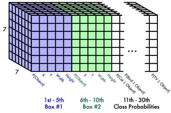
入力画像は7×7のセルに分割されています。
各セルに対して、2個のバウンディングボックス(BB)に関する情報があり、それが青い部分と緑色の部分です
情報の詳細は以下5つのデータです
- P(Object):「領域の存在確率」と呼ぶことにする。つまりこの値が高いと、物体領域としての信用度が高いということ。
- X:セルにおけるBBの中心X位置
- Y:セルにおけるBBの中心Y位置
- Width:画像におけるBBの幅
- Height:画像におけるBBの高さ
さらに各セルに対して、20個のクラス確率情報があります。図では白い部分で描かれています。
20種類の画像に対するそれぞれの確率で、今まで実施してきたGoogLeNetやGenderNetと同じです。
上記のデータは推論の結果 output という変数に入っています。
これを関数 filter_objects に代入します
# filter out all the objects/boxes that don't meet thresholdsfiltered_objs =
filter_objectsの第一引数に先程のoutputを渡しています。
output.astype(np.float32)というのは、データの型をfloat32に合わせているだけです。
第二引数は入力画像の幅、第三引数には入力画像の高さを渡しています。戻り値が filterd_objs という変数に入ります。
filter_objects関数については後で詳細を解説しますが、変数filterd_objsには、アルゴリズムで説明した「すっきりした情報」が入ります。
#display the filtered objects/boxes in a GUI window
display_objects_in_gui関数については後で詳細を解説しますが、「入力画像」と先程の「すっきりした情報」を使って可視化しています。
ウィンドウが開いて画像が表示されます。
main関数のその他の構文についての説明は、GoogLeNetやGenderNetとほぼ同じですので、ここでは割愛します。
(4) filter_objects関数
# the raw number of floats returned from the inference (GetResult())num_inference_results =
main関数のoutputはinference_resultという変数で受け取っています。ここではその配列の要素数を取得しています。
printで表示させてみると分かりますが1470要素あります。main関数のところで、推論データの資料を載せましたが、計算してみると一致します。
1470 = 7 × 7 × ( 2 × 5 + 20 )
# the 20 classes this network was trained onnetwork_classifications =
今回のTinyYoloで認識できるクラスの文字列リストです
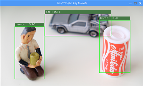
# only keep boxes with probabilities greater than thisprobability_threshold = 0.07
BBを表示させるかどうかを決める閾値です。自由に変更可能です。
数値が小さい程BBの表示数は増えますが、ノイズも増えてしまいます。
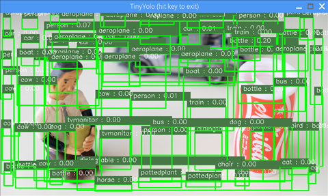
試しに 0.00 にしてみたときの画像です。
num_classifications = # should be 20grid_size = 7 # the image is a 7x7 grid. Each box in the grid is 64x64 pixelsboxes_per_grid_cell = 2 # the number of boxes returned for each grid cell
num_classificationsはクラス数です。20クラスです
grid_sizeはグリッドサイズ 7 です
boxes_per_grid_cellは1セルあたりのBBの数で2です
この3つは学習時に決まっている値であり、変更できません。
# grid_size is 7 (grid is 7x7)# num classifications is 20# boxes per grid cell is 2all_probabilities = np
np.zerosは全ての値を0にする関数で、all_probabilitiesを0で初期化しているという意味です。
all_probabilitiesは、全てのBBに対する「領域の存在確率」と「各画像クラスの確率」を掛け合わせた数値が入ります。
最終的に閾値probability_threshold(現状0.07)と比較して、BBを表示するか否かを決めます。
# classification_probabilities contains a probability for each classification for# each 64x64 pixel square of the grid. The source image contains# 7x7 of these 64x64 pixel squares and there are 20 possible classificationsclassification_probabilities = \npnum_of_class_probs =
classification_probabilitiesは「各画像クラスの確率」です
推論結果inference_resultから 980個の要素をスライスで取得しています。
980 - 0 = 7 × 7 × 20
# The probability scale factor for each boxbox_prob_scale_factor = np
box_prob_scale_factor はBBの「領域の存在確率」です。
推論結果inference_resultから 98個の要素をスライスで取得しています。
1078 - 980 = 7 × 7 × 2
# get the boxes from the results and adjust to be pixel unitsall_boxes = np
all_boxes はBBの位置情報です。
推論結果inference_resultから残りの要素をスライスで取得しています
1470 -1078 = 7 × 7 × 2 × 4
位置情報には以下の4つの情報が入っています。
- X:セルにおけるBBの中心X位置
- Y:セルにおけるBBの中心Y位置
- Width:画像におけるBBの幅
- Height:画像におけるBBの高さ
関数boxes_to_pixel_units に all_boxesを渡して中身を変換します
関数の詳細は別途解説しますが、簡単にいうとBBの位置情報を入力画像を基準とした具体的なピクセル座標に変換しています。
# adjust the probabilities with the scaling factorfor box_index in : # loop over boxesfor class_index in : # loop over classifications= np
0で初期化していた all_probabilities に「各画像クラスの確率」と「領域の存在確率」の掛け算を行った値を代入しています。この値のことを「BB確率」と呼ぶことにしましょう
probability_threshold_mask = npbox_threshold_mask = npboxes_above_threshold =classifications_for_boxes_above = npprobabilities_above_threshold =
ちょっと多いですが、一気に説明します。ポイントは閾値以下を取っ払っている点です。
probability_threshold_mask は all_probabilities で 閾値probability_threshold(現状0.07)以上のみをTrueとするマスクの配列
box_threshold_mask は 上記のTrueの要素のインデックスのみを集めた配列
boxes_above_threshold は 上記のTrueのみ(閾値以上のみ)のBB座標情報配列
classifications_for_boxes_above は box_threshold_mask においてクラス確率が最大のインデックス配列
probabilities_above_threshold は probability_threshold_mask においてTrueのみ(閾値以上のみ)の BB確率配列
# sort the boxes from highest probability to lowest and then# sort the probabilities and classifications to matchargsort = npboxes_above_threshold =classifications_for_boxes_above =probabilities_above_threshold =
続けて一気に説明します。ポイントはBB確率の大きい順に並べている点です。argsortのみが新規の変数で、それ以外の3つの変数は更新です。
argsort は probabilities_above_thresholdを降順に並べた配列
boxes_above_threshold は BB確率が大きい順に並べたBB座標情報配列(閾値以下は含まない)
classifications_for_boxes_above は BB確率が大きい順に並べたクラス確率が最大のインデックス配列(閾値以下は含まない)
probabilities_above_threshold は BB確率が大きい順に並べたBB確率配列(閾値以下は含まない)
# get mask for boxes that seem to be the same objectduplicate_box_mask =
関数get_duplicate_box_maskにboxes_above_thresholdを入れて、戻り値としてduplicate_box_maskを得ています
関数の詳細は別途解説しますが、簡単にいうと重複しているBBの除去です
# update the boxes, probabilities and classifications removing duplicates.boxes_above_threshold =classifications_for_boxes_above =probabilities_above_threshold =
各変数の更新です
boxes_above_threshold, classifications_for_boxes_above, probabilities_above_threshold について重複したBBを除去しています
classes_boxes_and_probs =for i in :classes_boxes_and_probsreturn classes_boxes_and_probs
classes_boxes_and_probsというリストを作成して、以下の内容を追加しています。最後にはこのリストを戻り値としてmain関数へ返しています。
- network_classifications[classifications_for_boxes_above[i]] : 分類文字列("car" や "person" など)
- boxes_above_threshold[i][0] : BBの中心X座標
- boxes_above_threshold[i][1] : BBの中心Y座標
- boxes_above_threshold[i][2] : BBの幅
- boxes_above_threshold[i][3] : BBの高さ
- probabilities_above_threshold[i] : BB確率
各配列は、BB確率が閾値以上で、BBの重複除去処理されていて、BB確率の大きい順に並んでいます。
(5) boxes_to_pixel_units関数
全コードを一気に説明します。
# number of boxes per grid cellboxes_per_cell = 2# setup some offset values to map boxes to pixels# box_offset will be [[ [0, 0], [1, 1], [2, 2], [3, 3], [4, 4], [5, 5], [6, 6]] ...repeated for 7 ]box_offset = np# adjust the box center+= box_offset+= np= / (grid_size * 1.0)# adjust the lengths and widths= np= np#scale the boxes to the image size in pixels*= image_width*= image_height*= image_width*= image_height
最初にオフセット用の配列box_offsetを作っています。2個セットになっている理由は、1セルに2つのBBがあるためです
"adjust the box center"ではオフセットを加算することで、中心位置をBB基準から全体入力画像の位置へ変換しています。grid_sizeで割っているのは0.0~1.0に正規化するためです。
"adjust the lengths and widths"では、widthとheightを二乗しています。実は元々のwidhtとheightのデータは平方根の値ということですね。
"scale the boxes to the image size in pixels"で、中心位置X,Yと幅,高さを正規化された値から、画像のピクセル座標値へ変換しています。
関数の戻り値がありませんが、Pythonで関数の引数でリストを渡した場合は「参照渡し」になります。つまりbox_listの値が変化することで、呼び出し元の filter_objects関数のall_boxesの値も変化しています。
(6) get_duplicate_box_mask関数
こちらも一気に説明します。
# The intersection-over-union threshold to use when determining duplicates.# objects/boxes found that are over this threshold will be# considered the same objectmax_iou = 0.35box_mask = npfor i in :if == 0: continuefor j in :if > max_iou:= 0.0filter_iou_mask = npreturn filter_iou_mask
引数box_listには、BB確率が大きい順に並べたBB座標情報配列(閾値以下は含まない)が入っています。
max_iouはこの関数でのみ使用する閾値です。iouはIntersection Over Unionの略で、get_intersection_over_union関数で詳細説明します。
各box_listを2つ選んで、get_intersection_over_union関数に渡し、結果が max_iou 以上の場合は 0.0 にしています。
戻り値として返すfilter_iou_maskには、max_iou未満を満たす配列のみが入ります。
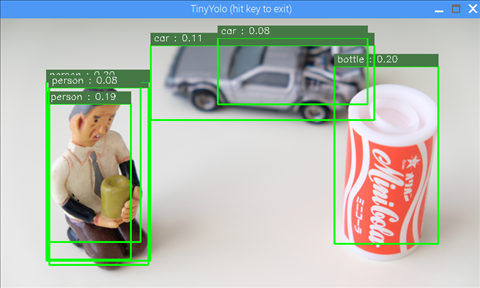
試しに max_iouを1.00 にしてみたときの画像です。
1.0だと全ての重なりを許可したのに等しく、get_duplicate_box_mask関数を行っていないことと同等になります。
(7) get_intersection_over_union関数
こちらも一気にいきます
# one diminsion of the intersecting boxintersection_dim_1 = -\# the other dimension of the intersecting boxintersection_dim_2 = -\if intersection_dim_1 < 0 or intersection_dim_2 < 0 :# no intersection areaintersection_area = 0else :# intersection area is product of intersection dimensionsintersection_area = intersection_dim_1*intersection_dim_2# calculate the union area which is the area of each box added# and then we need to subtract out the intersection area since# it is counted twice (by definition it is in each box)union_area = * + * - intersection_area;# now we can return the intersection over unioniou = intersection_area / union_areareturn iou
変数intersection_dim_1について、詳細確認します。
box_1[0]+0.5*box_1[2] は ボックス1の中心X座標 + 0.5 × ボックス1の幅 です。つまり、下の図でいうと a のX座標に相当します。
他も同様に、b, c, d のX座標に相当していることが分かると思います。
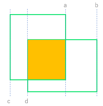
a, b, c, d を用いると intersection_dim_1 は以下のように書けます
intersection_dim_1 = -
minは小さい方、maxは大きい方を返しますので、最終的には a - d です。
つまりintersection_dim_1は、2つのボックスが重なった領域(黄色い領域)の幅のことです。
同様にintersection_dim_2は、2つのボックスが重なった領域(黄色い領域)の高さです。
途中のif文は、重なり領域が無い場合は変数intersection_areaに0を、重なり領域がある場合は変数intersection_areaにその面積を代入しています。
変数union_areaはボックス1の面積とボックス2の面積の和から重なり領域の面積を引いた面積です。
つまりiouとは、2つのボックスが重なっている割合を数値化したもので、数値が大きいほど重なり度合いが高いという意味になります。
最後に変数iouを返しています
(8) display_objects_in_gui関数
最後に display_objects_in_gui を簡単に説明します。
# copy image so we can draw on it. Could just draw directly on source image if not concerned about that.display_image = source_imagesource_image_width = source_image.shapesource_image_height = source_image.shapex_ratio = / NETWORK_IMAGE_WIDTHy_ratio = / NETWORK_IMAGE_HEIGHT
入力画像source_imageのコピーをdisplay_imageに代入します
source_image_widthは入力画像の幅、source_image_heightは入力画像の高さです
x_ratio, y_rationは 推論時の画像サイズとの比です。
# loop through each box and draw it on the image along with a classification labelprint('Found this many objects in the image: ' + )for obj_index in :center_x =center_y =half_width = //2half_height = //2# calculate box (left, top) and (right, bottom) coordinatesbox_left =box_top =box_right =box_bottom =print('box at index ' + + ' is... left: ' + + ', top: ' + + ', right: ' + + ', bottom: ' + )#draw the rectangle on the image. This is hopefully around the objectbox_color = (0, 255, 0) # green boxbox_thickness = 2cv2
for文の途中ですが、ここでやっていることは、入力画像の上にバウンディングボックスを描画しているという内容です。
# draw the classification label string just above and to the left of the rectanglelabel_background_color = (70, 120, 70) # greyish green background for textlabel_text_color = (255, 255, 255) # white textcv2cv2
こちらはバウンディングボックスの上に、クラスとBB確率のラベルを描画しているという内容です。ラベルは、塗りつぶしの矩形領域を描画後に、テキストを描画しています。
window_name = 'TinyYolo (hit key to exit)'cv2while (True):raw_key = cv2
何度か登場してきているOpenCVによる構文です。
ウィンドウに画像を表示して、キーが押されたら終了です。
# check if the window is visible, this means the user hasn't closed# the window via the X button (may only work with opencv 3.xprop_val = cv2if ((raw_key != -1) or (prop_val < 0.0)):# the user hit a key or closed the window (in that order)break
こちらはOpenCVのときに最後に説明した内容です。ウィンドウの閉じるボタンの対応です。
大変ボリュームが多くなってしまいましたが、TinyYoloのソースコード詳細を解説しました。じっくり読まれた方、大変お疲れさまでした。
次回はソースコードを改造して、TinyYoloでUSBカメラ入力によるリアルタイム化とAR描画に挑戦します!
以上、「TinyYoloで物体検出」でした。